[Mirror] Exploring Elliptic Curve Pairings
2017 Jan 14
See all posts
[Mirror] Exploring Elliptic Curve Pairings
This is a mirror of the post at https://medium.com/@VitalikButerin/exploring-elliptic-curve-pairings-c73c1864e627
Trigger warning: math.
One of the key cryptographic primitives behind various constructions, including deterministic threshold signatures, zk-SNARKs and other simpler forms of zero-knowledge proofs is the elliptic curve pairing. Elliptic curve pairings (or "bilinear maps") are a recent addition to a 30-year-long history of using elliptic curves for cryptographic applications including encryption and digital signatures; pairings introduce a form of "encrypted multiplication", greatly expanding what elliptic curve-based protocols can do. The purpose of this article will be to go into elliptic curve pairings in detail, and explain a general outline of how they work.
You're not expected to understand everything here the first time you read it, or even the tenth time; this stuff is genuinely hard. But hopefully this article will give you at least a bit of an idea as to what is going on under the hood.
Elliptic curves themselves are very much a nontrivial topic to understand, and this article will generally assume that you know how they work; if you do not, I recommend this article here as a primer: https://blog.cloudflare.com/a-relatively-easy-to-understand-primer-on-elliptic-curve-cryptography/. As a quick summary, elliptic curve cryptography involves mathematical objects called "points" (these are literal two-dimensional points with \((x, y)\) coordinates), with special formulas for adding and subtracting them (ie. for calculating the coordinates of \(R = P + Q\)), and you can also multiply a point by an integer (ie. \(P \cdot n = P + P + ... + P\), though there's a much faster way to compute it if \(n\) is big).
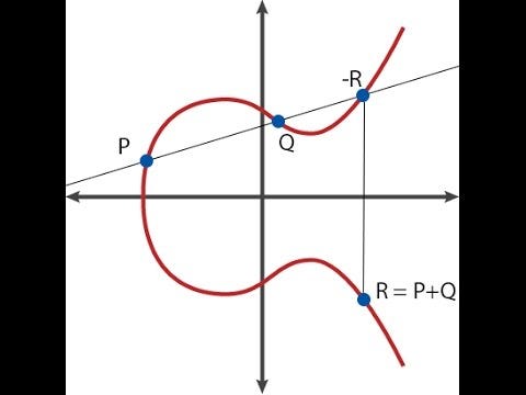
Here's how point addition looks like graphically.
There exists a special point called the "point at infinity" (\(O\)), the equivalent of zero in point arithmetic; it's always the case that \(P + O = P\). Also, a curve has an "order"; there exists a number \(n\) such that \(P \cdot n = O\) for any \(P\) (and of course, \(P \cdot (n+1) = P, P \cdot (7 \cdot n + 5) = P \cdot 5\), and so on). There is also some commonly agreed upon "generator point" \(G\), which is understood to in some sense represent the number \(1\). Theoretically, any point on a curve (except \(O\)) can be \(G\); all that matters is that \(G\) is standardized.
Pairings go a step further in that they allow you to check certain kinds of more complicated equations on elliptic curve points — for example, if \(P = G \cdot p, Q = G \cdot q\) and \(R = G \cdot r\), you can check whether or not \(p \cdot q = r\), having just \(P, Q\) and \(R\) as inputs. This might seem like the fundamental security guarantees of elliptic curves are being broken, as information about \(p\) is leaking from just knowing P, but it turns out that the leakage is highly contained — specifically, the decisional Diffie Hellman problem is easy, but the computational Diffie Hellman problem (knowing \(P\) and \(Q\) in the above example, computing \(R = G \cdot p \cdot q\)) and the discrete logarithm problem (recovering \(p\) from \(P\)) remain computationally infeasible (at least, if they were before).
A third way to look at what pairings do, and one that is perhaps most illuminating for most of the use cases that we are about, is that if you view elliptic curve points as one-way encrypted numbers (that is, \(encrypt(p) = p \cdot G = P\)), then whereas traditional elliptic curve math lets you check linear constraints on the numbers (eg. if \(P = G \cdot p, Q = G \cdot q\) and \(R = G \cdot r\), checking \(5 \cdot P + 7 \cdot Q = 11 \cdot R\) is really checking that \(5 \cdot p + 7 \cdot q = 11 \cdot r\)), pairings let you check quadratic constraints (eg. checking \(e(P, Q) \cdot e(G, G \cdot 5) = 1\) is really checking that \(p \cdot q + 5 = 0\)). And going up to quadratic is enough to let us work with deterministic threshold signatures, quadratic arithmetic programs and all that other good stuff.
Now, what is this funny \(e(P, Q)\) operator that we introduced above? This is the pairing. Mathematicians also sometimes call it a bilinear map; the word "bilinear" here basically means that it satisfies the constraints:
\(e(P, Q + R) = e(P, Q) \cdot e(P, R)\)
\(e(P + S, Q) = e(P, Q) \cdot e(S, Q)\)
Note that \(+\) and \(\cdot\) can be arbitrary operators; when you're creating fancy new kinds of mathematical objects, abstract algebra doesn't care how \(+\) and \(\cdot\) are defined, as long as they are consistent in the usual ways, eg. \(a + b = b + a, (a \cdot b) \cdot c = a \cdot (b \cdot c)\) and \((a \cdot c) + (b \cdot c) = (a + b) \cdot c\).
If \(P\), \(Q\), \(R\) and \(S\) were simple numbers, then making a simple pairing is easy: we can do \(e(x, y) = 2^{xy}\). Then, we can see:
\(e(3, 4+ 5) = 2^{3 \cdot 9} = 2^{27}\)
\(e(3, 4) \cdot e(3, 5) = 2^{3 \cdot 4} \cdot 2^{3 \cdot 5} = 2^{12} \cdot 2^{15} = 2^{27}\)
It's bilinear!
However, such simple pairings are not suitable for cryptography because the objects that they work on are simple integers and are too easy to analyze; integers make it easy to divide, compute logarithms, and make various other computations; simple integers have no concept of a "public key" or a "one-way function". Additionally, with the pairing described above you can go backwards - knowing \(x\), and knowing \(e(x, y)\), you can simply compute a division and a logarithm to determine \(y\). We want mathematical objects that are as close as possible to "black boxes", where you can add, subtract, multiply and divide, but do nothing else. This is where elliptic curves and elliptic curve pairings come in.
It turns out that it is possible to make a bilinear map over elliptic curve points — that is, come up with a function \(e(P, Q)\) where the inputs \(P\) and \(Q\) are elliptic curve points, and where the output is what's called an \((F_p)^{12}\) element (at least in the specific case we will cover here; the specifics differ depending on the details of the curve, more on this later), but the math behind doing so is quite complex.
First, let's cover prime fields and extension fields. The pretty elliptic curve in the picture earlier in this post only looks that way if you assume that the curve equation is defined using regular real numbers. However, if we actually use regular real numbers in cryptography, then you can use logarithms to "go backwards", and everything breaks; additionally, the amount of space needed to actually store and represent the numbers may grow arbitrarily. Hence, we instead use numbers in a prime field.
A prime field consists of the set of numbers \(0, 1, 2... p-1\), where \(p\) is prime, and the various operations are defined as follows:
\(a + b: (a + b)\) % \(p\)
\(a \cdot b: (a \cdot b)\) % \(p\)
\(a - b: (a - b)\) % \(p\)
\(a / b: (a \cdot b^{p-2})\) % \(p\)
Basically, all math is done modulo \(p\) (see here for an introduction to modular math). Division is a special case; normally, \(\frac{3}{2}\) is not an integer, and here we want to deal only with integers, so we instead try to find the number \(x\) such that \(x \cdot 2 = 3\), where \(\cdot\) of course refers to modular multiplication as defined above. Thanks to Fermat's little theorem, the exponentiation trick shown above does the job, but there is also a faster way to do it, using the Extended Euclidean Algorithm. Suppose \(p = 7\); here are a few examples:
\(2 + 3 = 5\) % \(7 = 5\)
\(4 + 6 = 10\) % \(7 = 3\)
\(2 - 5 = -3\) % \(7 = 4\)
\(6 \cdot 3 = 18\) % \(7 = 4\)
\(3 / 2 = (3 \cdot 2^5)\) % \(7 = 5\)
\(5 \cdot 2 = 10\) % \(7 = 3\)
If you play around with this kind of math, you'll notice that it's perfectly consistent and satisfies all of the usual rules. The last two examples above show how \((a / b) \cdot b = a\); you can also see that \((a + b) + c = a + (b + c), (a + b) \cdot c = a \cdot c + b \cdot c\), and all the other high school algebraic identities you know and love continue to hold true as well. In elliptic curves in reality, the points and equations are usually computed in prime fields.
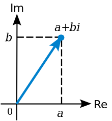
Now, let's talk about extension fields. You have probably already seen an extension field before; the most common example that you encounter in math textbooks is the field of complex numbers, where the field of real numbers is "extended" with the additional element \(\sqrt{-1} = i\). Basically, extension fields work by taking an existing field, then "inventing" a new element and defining the relationship between that element and existing elements (in this case, \(i^2 + 1 = 0\)), making sure that this equation does not hold true for any number that is in the original field, and looking at the set of all linear combinations of elements of the original field and the new element that you have just created.
We can do extensions of prime fields too; for example, we can extend the prime field \(\bmod 7\) that we described above with \(i\), and then we can do:
\((2 + 3i) + (4 + 2i) = 6 + 5i\)
\((5 + 2i) + 3 = 1 + 2i\)
\((6 + 2i) \cdot 2 = 5 + 4i\)
\(4i \cdot (2 + i) = 3 + i\)
That last result may be a bit hard to figure out; what happened there was that we first decompose the product into \(4i \cdot 2 + 4i \cdot i\), which gives \(8i - 4\), and then because we are working in \(\bmod 7\) math that becomes \(i + 3\). To divide, we do:
\(a / b: (a \cdot b^{(p^{2-2})})\) % \(p\)
Note that the exponent for Fermat's little theorem is now \(p^2\) instead of \(p\), though once again if we want to be more efficient we can also instead extend the Extended Euclidean Algorithm to do the job. Note that \(x^{p^2 - 1} = 1\) for any \(x\) in this field, so we call \(p^2 - 1\) the "order of the multiplicative group in the field".
With real numbers, the Fundamental Theorem of Algebra ensures that the quadratic extension that we call the complex numbers is "complete" — you cannot extend it further, because for any mathematical relationship (at least, any mathematical relationship defined by an algebraic formula) that you can come up with between some new element \(j\) and the existing complex numbers, it's possible to come up with at least one complex number that already satisfies that relationship. With prime fields, however, we do not have this issue, and so we can go further and make cubic extensions (where the mathematical relationship between some new element \(w\) and existing field elements is a cubic equation, so \(1, w\) and \(w^2\) are all linearly independent of each other), higher-order extensions, extensions of extensions, etc. And it is these kinds of supercharged modular complex numbers that elliptic curve pairings are built on.
For those interested in seeing the exact math involved in making all of these operations written out in code, prime fields and field extensions are implemented here: https://github.com/ethereum/py_pairing/blob/e95dece17e5d948e62b1492b05ba88b726aa25e6/py_ecc/bn128/bn128_field_elements.py
Now, on to elliptic curve pairings. An elliptic curve pairing (or rather, the specific form of pairing we'll explore here; there are also other types of pairings, though their logic is fairly similar) is a map \(G_2 \times G_1 \rightarrow G_t\), where:
\(\bf G_1\) is an elliptic curve, where points satisfy an equation of the form \(y^2 = x^3 + b\), and where both coordinates are elements of \(F_p\) (ie. they are simple numbers, except arithmetic is all done modulo some prime number)
\(\bf G_2\) is an elliptic curve, where points satisfy the same equation as \(G_1\), except where the coordinates are elements of \((F_p)^{12}\) (ie. they are the supercharged complex numbers we talked about above; we define a new "magic number" \(w\), which is defined by a \(12\)th degree polynomial like \(w^{12} - 18 \cdot w^6 + 82 = 0\))
\(\bf G_t\) is the type of object that the result of the elliptic curve goes into. In the curves that we look at, \(G_t\) is \(\bf (F_p)^{12}\) (the same supercharged complex number as used in \(G_2\))
The main property that it must satisfy is bilinearity, which in this context means that:
\(e(P, Q + R) = e(P, Q) \cdot e(P, R)\)
\(e(P + Q, R) = e(P, R) \cdot e(Q, R)\)
There are two other important criteria:
Efficient computability (eg. we can make an easy pairing by simply taking the discrete logarithms of all points and multiplying them together, but this is as computationally hard as breaking elliptic curve cryptography in the first place, so it doesn't count)
Non-degeneracy (sure, you could just define \(e(P, Q) = 1\), but that's not a particularly useful pairing)
So how do we do this?
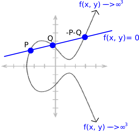
The math behind why pairing functions work is quite tricky and involves quite a bit of advanced algebra going even beyond what we've seen so far, but I'll provide an outline. First of all, we need to define the concept of a divisor, basically an alternative way of representing functions on elliptic curve points. A divisor of a function basically counts the zeroes and the infinities of the function. To see what this means, let's go through a few examples. Let us fix some point \(P = (P_x, P_y)\), and consider the following function:
\(f(x, y) = x - P_x\)
The divisor is \([P] + [-P] - 2 \cdot [O]\) (the square brackets are used to represent the fact that we are referring to the presence of the point \(P\) in the set of zeroes and infinities of the function, not the point P itself; \([P] + [Q]\) is not the same thing as \([P + Q]\)). The reasoning is as follows:
The function is equal to zero at \(P\), since \(x\) is \(P_x\), so \(x - P_x = 0\)
The function is equal to zero at \(-P\), since \(-P\) and \(P\) share the same \(x\) coordinate
The function goes to infinity as \(x\) goes to infinity, so we say the function is equal to infinity at \(O\). There's a technical reason why this infinity needs to be counted twice, so \(O\) gets added with a "multiplicity" of \(-2\) (negative because it's an infinity and not a zero, two because of this double counting).
The technical reason is roughly this: because the equation of the curve is \(x^3 = y^2 + b, y\) goes to infinity "\(1.5\) times faster" than \(x\) does in order for \(y^2\) to keep up with \(x^3\); hence, if a linear function includes only \(x\) then it is represented as an infinity of multiplicity \(2\), but if it includes \(y\) then it is represented as an infinity of multiplicity \(3\).
Now, consider a "line function":
\(ax + by + c = 0\)
Where \(a\), \(b\) and \(c\) are carefully chosen so that the line passes through points \(P\) and \(Q\). Because of how elliptic curve addition works (see the diagram at the top), this also means that it passes through \(-P-Q\). And it goes up to infinity dependent on both \(x\) and \(y\), so the divisor becomes \([P]+ [Q] + [-P-Q] - 3 \cdot [O]\).
We know that every "rational function" (ie. a function defined only using a finite number of \(+, -, \cdot\) and \(/\) operations on the coordinates of the point) uniquely corresponds to some divisor, up to multiplication by a constant (ie. if two functions \(F\) and \(G\) have the same divisor, then \(F = G \cdot k\) for some constant \(k\)).
For any two functions \(F\) and \(G\), the divisor of \(F \cdot G\) is equal to the divisor of \(F\) plus the divisor of \(G\) (in math textbooks, you'll see \((F \cdot G) = (F) + (G)\)), so for example if \(f(x, y) = P_x - x\), then \((f^3) = 3 \cdot [P] + 3 \cdot [-P] - 6 \cdot [O]\); \(P\) and \(-P\) are "triple-counted" to account for the fact that \(f^3\) approaches \(0\) at those points "three times as quickly" in a certain mathematical sense.
Note that there is a theorem that states that if you "remove the square brackets" from a divisor of a function, the points must add up to \(O ([P] + [Q] + [-P-Q] - 3 \cdot [O]\) clearly fits, as \(P + Q - P - Q - 3 \cdot O = O)\), and any divisor that has this property is the divisor of a function.
Now, we're ready to look at Tate pairings. Consider the following functions, defined via their divisors:
\((F_P) = n \cdot [P] - n \cdot [O]\), where \(n\) is the order of \(G_1\), ie. \(n \cdot P = O\) for any \(P\)
\((F_Q) = n \cdot [Q] - n \cdot [O]\)
\((g) = [P + Q] - [P] - [Q] + [O]\)
Now, let's look at the product \(F_P \cdot F_Q \cdot g^n\). The divisor is:
\(n \cdot [P] - n \cdot [O] + n \cdot [Q] - n \cdot [O] + n \cdot [P + Q] - n \cdot [P] - n \cdot [Q] + n \cdot [O]\)
Which simplifies neatly to:
\(n \cdot [P + Q] - n \cdot [O]\)
Notice that this divisor is of exactly the same format as the divisor for \(F_P\) and \(F_Q\) above. Hence, \(F_P \cdot F_Q \cdot g^n = F_{P + Q}\).
Now, we introduce a procedure called the "final exponentiation" step, where we take the result of our functions above (\(F_P, F_Q\), etc.) and raise it to the power \(z = (p^{12} - 1) / n\), where \(p^{12} - 1\) is the order of the multiplicative group in \((F_p)^{12}\) (ie. for any \(x \in (F_p)^{12}, x^{(p^{12} - 1)} = 1\)). Notice that if you apply this exponentiation to any result that has already been raised to the power of \(n\), you get an exponentiation to the power of \(p^{12} - 1\), so the result turns into \(1\). Hence, after final exponentiation, \(g^n\) cancels out and we get \(F_P^z \cdot F_Q^z = (F_{P + Q})^z\). There's some bilinearity for you.
Now, if you want to make a function that's bilinear in both arguments, you need to go into spookier math, where instead of taking \(F_P\) of a value directly, you take \(F_P\) of a divisor, and that's where the full "Tate pairing" comes from. To prove some more results you have to deal with notions like "linear equivalence" and "Weil reciprocity", and the rabbit hole goes on from there. You can find more reading material on all of this here and here.
For an implementation of a modified version of the Tate pairing, called the optimal Ate paring, see here. The code implements Miller's algorithm, which is needed to actually compute \(F_P\).
Note that the fact pairings like this are possible is somewhat of a mixed blessing: on the one hand, it means that all the protocols we can do with pairings become possible, but is also means that we have to be more careful about what elliptic curves we use.
Every elliptic curve has a value called an embedding degree; essentially, the smallest \(k\) such that \(p^k - 1\) is a multiple of \(n\) (where \(p\) is the prime used for the field and \(n\) is the curve order). In the fields above, \(k = 12\), and in the fields used for traditional ECC (ie. where we don't care about pairings), the embedding degree is often extremely large, to the point that pairings are computationally infeasible to compute; however, if we are not careful then we can generate fields where \(k = 4\) or even \(1\).
If \(k = 1\), then the "discrete logarithm" problem for elliptic curves (essentially, recovering \(p\) knowing only the point \(P = G \cdot p\), the problem that you have to solve to "crack" an elliptic curve private key) can be reduced into a similar math problem over \(F_p\), where the problem becomes much easier (this is called the MOV attack); using curves with an embedding degree of \(12\) or higher ensures that this reduction is either unavailable, or that solving the discrete log problem over pairing results is at least as hard as recovering a private key from a public key "the normal way" (ie. computationally infeasible). Do not worry; all standard curve parameters have been thoroughly checked for this issue.
Stay tuned for a mathematical explanation of how zk-SNARKs work, coming soon.
Special thanks to Christian Reitwiessner, Ariel Gabizon (from Zcash) and Alfred Menezes for reviewing and making corrections.
[Mirror] Exploring Elliptic Curve Pairings
2017 Jan 14 See all postsThis is a mirror of the post at https://medium.com/@VitalikButerin/exploring-elliptic-curve-pairings-c73c1864e627
Trigger warning: math.
One of the key cryptographic primitives behind various constructions, including deterministic threshold signatures, zk-SNARKs and other simpler forms of zero-knowledge proofs is the elliptic curve pairing. Elliptic curve pairings (or "bilinear maps") are a recent addition to a 30-year-long history of using elliptic curves for cryptographic applications including encryption and digital signatures; pairings introduce a form of "encrypted multiplication", greatly expanding what elliptic curve-based protocols can do. The purpose of this article will be to go into elliptic curve pairings in detail, and explain a general outline of how they work.
You're not expected to understand everything here the first time you read it, or even the tenth time; this stuff is genuinely hard. But hopefully this article will give you at least a bit of an idea as to what is going on under the hood.
Elliptic curves themselves are very much a nontrivial topic to understand, and this article will generally assume that you know how they work; if you do not, I recommend this article here as a primer: https://blog.cloudflare.com/a-relatively-easy-to-understand-primer-on-elliptic-curve-cryptography/. As a quick summary, elliptic curve cryptography involves mathematical objects called "points" (these are literal two-dimensional points with \((x, y)\) coordinates), with special formulas for adding and subtracting them (ie. for calculating the coordinates of \(R = P + Q\)), and you can also multiply a point by an integer (ie. \(P \cdot n = P + P + ... + P\), though there's a much faster way to compute it if \(n\) is big).
Here's how point addition looks like graphically.
There exists a special point called the "point at infinity" (\(O\)), the equivalent of zero in point arithmetic; it's always the case that \(P + O = P\). Also, a curve has an "order"; there exists a number \(n\) such that \(P \cdot n = O\) for any \(P\) (and of course, \(P \cdot (n+1) = P, P \cdot (7 \cdot n + 5) = P \cdot 5\), and so on). There is also some commonly agreed upon "generator point" \(G\), which is understood to in some sense represent the number \(1\). Theoretically, any point on a curve (except \(O\)) can be \(G\); all that matters is that \(G\) is standardized.
Pairings go a step further in that they allow you to check certain kinds of more complicated equations on elliptic curve points — for example, if \(P = G \cdot p, Q = G \cdot q\) and \(R = G \cdot r\), you can check whether or not \(p \cdot q = r\), having just \(P, Q\) and \(R\) as inputs. This might seem like the fundamental security guarantees of elliptic curves are being broken, as information about \(p\) is leaking from just knowing P, but it turns out that the leakage is highly contained — specifically, the decisional Diffie Hellman problem is easy, but the computational Diffie Hellman problem (knowing \(P\) and \(Q\) in the above example, computing \(R = G \cdot p \cdot q\)) and the discrete logarithm problem (recovering \(p\) from \(P\)) remain computationally infeasible (at least, if they were before).
A third way to look at what pairings do, and one that is perhaps most illuminating for most of the use cases that we are about, is that if you view elliptic curve points as one-way encrypted numbers (that is, \(encrypt(p) = p \cdot G = P\)), then whereas traditional elliptic curve math lets you check linear constraints on the numbers (eg. if \(P = G \cdot p, Q = G \cdot q\) and \(R = G \cdot r\), checking \(5 \cdot P + 7 \cdot Q = 11 \cdot R\) is really checking that \(5 \cdot p + 7 \cdot q = 11 \cdot r\)), pairings let you check quadratic constraints (eg. checking \(e(P, Q) \cdot e(G, G \cdot 5) = 1\) is really checking that \(p \cdot q + 5 = 0\)). And going up to quadratic is enough to let us work with deterministic threshold signatures, quadratic arithmetic programs and all that other good stuff.
Now, what is this funny \(e(P, Q)\) operator that we introduced above? This is the pairing. Mathematicians also sometimes call it a bilinear map; the word "bilinear" here basically means that it satisfies the constraints:
\(e(P, Q + R) = e(P, Q) \cdot e(P, R)\)
\(e(P + S, Q) = e(P, Q) \cdot e(S, Q)\)
Note that \(+\) and \(\cdot\) can be arbitrary operators; when you're creating fancy new kinds of mathematical objects, abstract algebra doesn't care how \(+\) and \(\cdot\) are defined, as long as they are consistent in the usual ways, eg. \(a + b = b + a, (a \cdot b) \cdot c = a \cdot (b \cdot c)\) and \((a \cdot c) + (b \cdot c) = (a + b) \cdot c\).
If \(P\), \(Q\), \(R\) and \(S\) were simple numbers, then making a simple pairing is easy: we can do \(e(x, y) = 2^{xy}\). Then, we can see:
\(e(3, 4+ 5) = 2^{3 \cdot 9} = 2^{27}\)
\(e(3, 4) \cdot e(3, 5) = 2^{3 \cdot 4} \cdot 2^{3 \cdot 5} = 2^{12} \cdot 2^{15} = 2^{27}\)
It's bilinear!
However, such simple pairings are not suitable for cryptography because the objects that they work on are simple integers and are too easy to analyze; integers make it easy to divide, compute logarithms, and make various other computations; simple integers have no concept of a "public key" or a "one-way function". Additionally, with the pairing described above you can go backwards - knowing \(x\), and knowing \(e(x, y)\), you can simply compute a division and a logarithm to determine \(y\). We want mathematical objects that are as close as possible to "black boxes", where you can add, subtract, multiply and divide, but do nothing else. This is where elliptic curves and elliptic curve pairings come in.
It turns out that it is possible to make a bilinear map over elliptic curve points — that is, come up with a function \(e(P, Q)\) where the inputs \(P\) and \(Q\) are elliptic curve points, and where the output is what's called an \((F_p)^{12}\) element (at least in the specific case we will cover here; the specifics differ depending on the details of the curve, more on this later), but the math behind doing so is quite complex.
First, let's cover prime fields and extension fields. The pretty elliptic curve in the picture earlier in this post only looks that way if you assume that the curve equation is defined using regular real numbers. However, if we actually use regular real numbers in cryptography, then you can use logarithms to "go backwards", and everything breaks; additionally, the amount of space needed to actually store and represent the numbers may grow arbitrarily. Hence, we instead use numbers in a prime field.
A prime field consists of the set of numbers \(0, 1, 2... p-1\), where \(p\) is prime, and the various operations are defined as follows:
\(a + b: (a + b)\) % \(p\)
\(a \cdot b: (a \cdot b)\) % \(p\)
\(a - b: (a - b)\) % \(p\)
\(a / b: (a \cdot b^{p-2})\) % \(p\)
Basically, all math is done modulo \(p\) (see here for an introduction to modular math). Division is a special case; normally, \(\frac{3}{2}\) is not an integer, and here we want to deal only with integers, so we instead try to find the number \(x\) such that \(x \cdot 2 = 3\), where \(\cdot\) of course refers to modular multiplication as defined above. Thanks to Fermat's little theorem, the exponentiation trick shown above does the job, but there is also a faster way to do it, using the Extended Euclidean Algorithm. Suppose \(p = 7\); here are a few examples:
\(2 + 3 = 5\) % \(7 = 5\)
\(4 + 6 = 10\) % \(7 = 3\)
\(2 - 5 = -3\) % \(7 = 4\)
\(6 \cdot 3 = 18\) % \(7 = 4\)
\(3 / 2 = (3 \cdot 2^5)\) % \(7 = 5\)
\(5 \cdot 2 = 10\) % \(7 = 3\)
If you play around with this kind of math, you'll notice that it's perfectly consistent and satisfies all of the usual rules. The last two examples above show how \((a / b) \cdot b = a\); you can also see that \((a + b) + c = a + (b + c), (a + b) \cdot c = a \cdot c + b \cdot c\), and all the other high school algebraic identities you know and love continue to hold true as well. In elliptic curves in reality, the points and equations are usually computed in prime fields.
Now, let's talk about extension fields. You have probably already seen an extension field before; the most common example that you encounter in math textbooks is the field of complex numbers, where the field of real numbers is "extended" with the additional element \(\sqrt{-1} = i\). Basically, extension fields work by taking an existing field, then "inventing" a new element and defining the relationship between that element and existing elements (in this case, \(i^2 + 1 = 0\)), making sure that this equation does not hold true for any number that is in the original field, and looking at the set of all linear combinations of elements of the original field and the new element that you have just created.
We can do extensions of prime fields too; for example, we can extend the prime field \(\bmod 7\) that we described above with \(i\), and then we can do:
\((2 + 3i) + (4 + 2i) = 6 + 5i\)
\((5 + 2i) + 3 = 1 + 2i\)
\((6 + 2i) \cdot 2 = 5 + 4i\)
\(4i \cdot (2 + i) = 3 + i\)
That last result may be a bit hard to figure out; what happened there was that we first decompose the product into \(4i \cdot 2 + 4i \cdot i\), which gives \(8i - 4\), and then because we are working in \(\bmod 7\) math that becomes \(i + 3\). To divide, we do:
\(a / b: (a \cdot b^{(p^{2-2})})\) % \(p\)
Note that the exponent for Fermat's little theorem is now \(p^2\) instead of \(p\), though once again if we want to be more efficient we can also instead extend the Extended Euclidean Algorithm to do the job. Note that \(x^{p^2 - 1} = 1\) for any \(x\) in this field, so we call \(p^2 - 1\) the "order of the multiplicative group in the field".
With real numbers, the Fundamental Theorem of Algebra ensures that the quadratic extension that we call the complex numbers is "complete" — you cannot extend it further, because for any mathematical relationship (at least, any mathematical relationship defined by an algebraic formula) that you can come up with between some new element \(j\) and the existing complex numbers, it's possible to come up with at least one complex number that already satisfies that relationship. With prime fields, however, we do not have this issue, and so we can go further and make cubic extensions (where the mathematical relationship between some new element \(w\) and existing field elements is a cubic equation, so \(1, w\) and \(w^2\) are all linearly independent of each other), higher-order extensions, extensions of extensions, etc. And it is these kinds of supercharged modular complex numbers that elliptic curve pairings are built on.
For those interested in seeing the exact math involved in making all of these operations written out in code, prime fields and field extensions are implemented here: https://github.com/ethereum/py_pairing/blob/e95dece17e5d948e62b1492b05ba88b726aa25e6/py_ecc/bn128/bn128_field_elements.py
Now, on to elliptic curve pairings. An elliptic curve pairing (or rather, the specific form of pairing we'll explore here; there are also other types of pairings, though their logic is fairly similar) is a map \(G_2 \times G_1 \rightarrow G_t\), where:
\(\bf G_1\) is an elliptic curve, where points satisfy an equation of the form \(y^2 = x^3 + b\), and where both coordinates are elements of \(F_p\) (ie. they are simple numbers, except arithmetic is all done modulo some prime number)
\(\bf G_2\) is an elliptic curve, where points satisfy the same equation as \(G_1\), except where the coordinates are elements of \((F_p)^{12}\) (ie. they are the supercharged complex numbers we talked about above; we define a new "magic number" \(w\), which is defined by a \(12\)th degree polynomial like \(w^{12} - 18 \cdot w^6 + 82 = 0\))
\(\bf G_t\) is the type of object that the result of the elliptic curve goes into. In the curves that we look at, \(G_t\) is \(\bf (F_p)^{12}\) (the same supercharged complex number as used in \(G_2\))
The main property that it must satisfy is bilinearity, which in this context means that:
\(e(P, Q + R) = e(P, Q) \cdot e(P, R)\)
\(e(P + Q, R) = e(P, R) \cdot e(Q, R)\)
There are two other important criteria:
Efficient computability (eg. we can make an easy pairing by simply taking the discrete logarithms of all points and multiplying them together, but this is as computationally hard as breaking elliptic curve cryptography in the first place, so it doesn't count)
Non-degeneracy (sure, you could just define \(e(P, Q) = 1\), but that's not a particularly useful pairing)
So how do we do this?
The math behind why pairing functions work is quite tricky and involves quite a bit of advanced algebra going even beyond what we've seen so far, but I'll provide an outline. First of all, we need to define the concept of a divisor, basically an alternative way of representing functions on elliptic curve points. A divisor of a function basically counts the zeroes and the infinities of the function. To see what this means, let's go through a few examples. Let us fix some point \(P = (P_x, P_y)\), and consider the following function:
\(f(x, y) = x - P_x\)
The divisor is \([P] + [-P] - 2 \cdot [O]\) (the square brackets are used to represent the fact that we are referring to the presence of the point \(P\) in the set of zeroes and infinities of the function, not the point P itself; \([P] + [Q]\) is not the same thing as \([P + Q]\)). The reasoning is as follows:
The function is equal to zero at \(P\), since \(x\) is \(P_x\), so \(x - P_x = 0\)
The function is equal to zero at \(-P\), since \(-P\) and \(P\) share the same \(x\) coordinate
The function goes to infinity as \(x\) goes to infinity, so we say the function is equal to infinity at \(O\). There's a technical reason why this infinity needs to be counted twice, so \(O\) gets added with a "multiplicity" of \(-2\) (negative because it's an infinity and not a zero, two because of this double counting).
The technical reason is roughly this: because the equation of the curve is \(x^3 = y^2 + b, y\) goes to infinity "\(1.5\) times faster" than \(x\) does in order for \(y^2\) to keep up with \(x^3\); hence, if a linear function includes only \(x\) then it is represented as an infinity of multiplicity \(2\), but if it includes \(y\) then it is represented as an infinity of multiplicity \(3\).
Now, consider a "line function":
\(ax + by + c = 0\)
Where \(a\), \(b\) and \(c\) are carefully chosen so that the line passes through points \(P\) and \(Q\). Because of how elliptic curve addition works (see the diagram at the top), this also means that it passes through \(-P-Q\). And it goes up to infinity dependent on both \(x\) and \(y\), so the divisor becomes \([P]+ [Q] + [-P-Q] - 3 \cdot [O]\).
We know that every "rational function" (ie. a function defined only using a finite number of \(+, -, \cdot\) and \(/\) operations on the coordinates of the point) uniquely corresponds to some divisor, up to multiplication by a constant (ie. if two functions \(F\) and \(G\) have the same divisor, then \(F = G \cdot k\) for some constant \(k\)).
For any two functions \(F\) and \(G\), the divisor of \(F \cdot G\) is equal to the divisor of \(F\) plus the divisor of \(G\) (in math textbooks, you'll see \((F \cdot G) = (F) + (G)\)), so for example if \(f(x, y) = P_x - x\), then \((f^3) = 3 \cdot [P] + 3 \cdot [-P] - 6 \cdot [O]\); \(P\) and \(-P\) are "triple-counted" to account for the fact that \(f^3\) approaches \(0\) at those points "three times as quickly" in a certain mathematical sense.
Note that there is a theorem that states that if you "remove the square brackets" from a divisor of a function, the points must add up to \(O ([P] + [Q] + [-P-Q] - 3 \cdot [O]\) clearly fits, as \(P + Q - P - Q - 3 \cdot O = O)\), and any divisor that has this property is the divisor of a function.
Now, we're ready to look at Tate pairings. Consider the following functions, defined via their divisors:
\((F_P) = n \cdot [P] - n \cdot [O]\), where \(n\) is the order of \(G_1\), ie. \(n \cdot P = O\) for any \(P\)
\((F_Q) = n \cdot [Q] - n \cdot [O]\)
\((g) = [P + Q] - [P] - [Q] + [O]\)
Now, let's look at the product \(F_P \cdot F_Q \cdot g^n\). The divisor is:
\(n \cdot [P] - n \cdot [O] + n \cdot [Q] - n \cdot [O] + n \cdot [P + Q] - n \cdot [P] - n \cdot [Q] + n \cdot [O]\)
Which simplifies neatly to:
\(n \cdot [P + Q] - n \cdot [O]\)
Notice that this divisor is of exactly the same format as the divisor for \(F_P\) and \(F_Q\) above. Hence, \(F_P \cdot F_Q \cdot g^n = F_{P + Q}\).
Now, we introduce a procedure called the "final exponentiation" step, where we take the result of our functions above (\(F_P, F_Q\), etc.) and raise it to the power \(z = (p^{12} - 1) / n\), where \(p^{12} - 1\) is the order of the multiplicative group in \((F_p)^{12}\) (ie. for any \(x \in (F_p)^{12}, x^{(p^{12} - 1)} = 1\)). Notice that if you apply this exponentiation to any result that has already been raised to the power of \(n\), you get an exponentiation to the power of \(p^{12} - 1\), so the result turns into \(1\). Hence, after final exponentiation, \(g^n\) cancels out and we get \(F_P^z \cdot F_Q^z = (F_{P + Q})^z\). There's some bilinearity for you.
Now, if you want to make a function that's bilinear in both arguments, you need to go into spookier math, where instead of taking \(F_P\) of a value directly, you take \(F_P\) of a divisor, and that's where the full "Tate pairing" comes from. To prove some more results you have to deal with notions like "linear equivalence" and "Weil reciprocity", and the rabbit hole goes on from there. You can find more reading material on all of this here and here.
For an implementation of a modified version of the Tate pairing, called the optimal Ate paring, see here. The code implements Miller's algorithm, which is needed to actually compute \(F_P\).
Note that the fact pairings like this are possible is somewhat of a mixed blessing: on the one hand, it means that all the protocols we can do with pairings become possible, but is also means that we have to be more careful about what elliptic curves we use.
Every elliptic curve has a value called an embedding degree; essentially, the smallest \(k\) such that \(p^k - 1\) is a multiple of \(n\) (where \(p\) is the prime used for the field and \(n\) is the curve order). In the fields above, \(k = 12\), and in the fields used for traditional ECC (ie. where we don't care about pairings), the embedding degree is often extremely large, to the point that pairings are computationally infeasible to compute; however, if we are not careful then we can generate fields where \(k = 4\) or even \(1\).
If \(k = 1\), then the "discrete logarithm" problem for elliptic curves (essentially, recovering \(p\) knowing only the point \(P = G \cdot p\), the problem that you have to solve to "crack" an elliptic curve private key) can be reduced into a similar math problem over \(F_p\), where the problem becomes much easier (this is called the MOV attack); using curves with an embedding degree of \(12\) or higher ensures that this reduction is either unavailable, or that solving the discrete log problem over pairing results is at least as hard as recovering a private key from a public key "the normal way" (ie. computationally infeasible). Do not worry; all standard curve parameters have been thoroughly checked for this issue.
Stay tuned for a mathematical explanation of how zk-SNARKs work, coming soon.
Special thanks to Christian Reitwiessner, Ariel Gabizon (from Zcash) and Alfred Menezes for reviewing and making corrections.